Note
Go to the end to download the full example code.
Consecutive submodeling with MAPDL pool#
- Problem description:
In this example, we demonstrate how to use MAPDL pool to perform a consecutive submodeling simulation with MAPDL and DPF.
- Analysis type:
Static Analysis
- Material properties:
Young’s modulus, \(E = 200 \, GPa\)
Poisson’s ratio, \(\mu = 0.3\)
- Boundary conditions (global model):
Fixed support applied at the bottom side
Frictionless support applied at the right side
- Loading:
Total displacement of -1 mm in the Y-direction at the top surface, ramped linearly over 10 timesteps
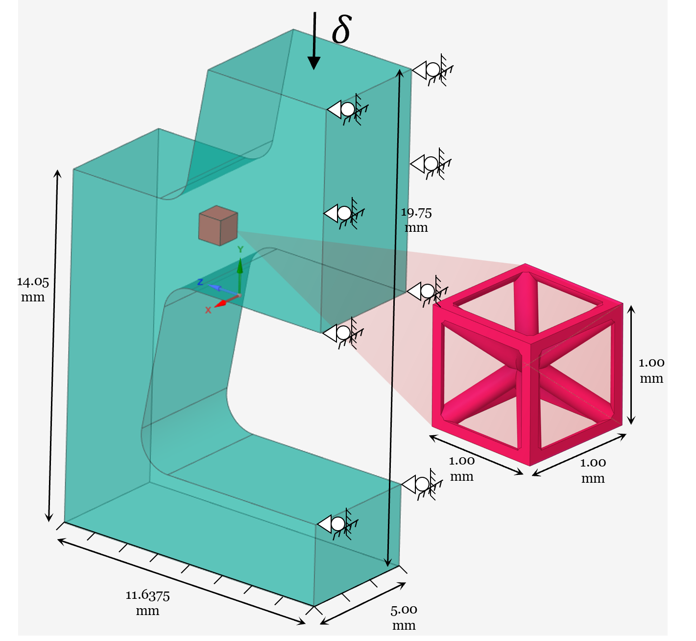
Problem sketch#
- Modeling notes:
At each timestep, the global model is solved with the specified boundary conditions; the resulting nodal displacements are interpolated to the boundary nodes of the local model, using the DPF interpolation operator. Those displacements are enforced as constraints to the local model, which is then solved, completing that timestep.
import os
from pathlib import Path
import shutil
import time as tt

from ansys.dpf import core as dpf
from ansys.mapdl.core import MapdlPool
from ansys.mapdl.core.examples.downloads import download_example_data
import numpy as np
Create directories to save the results#
folders = ["./outputs/mapdl-dpf/global", "./outputs/mapdl-dpf/local"]
for fdr in folders:
    shutil.rmtree(fdr, ignore_errors=True)
    Path(fdr).mkdir(parents=True, exist_ok=True)

# ##############################################################################
# Create a pool of MAPDL instances
# ~~~~~~~~~~~~~~~~~~~~~~~~~~~~~~~~
# We use the ``MapdlPool`` class to create two separate instances: one dedicated to
# the global simulation and the other to the local simulation

port_0 = int(os.getenv("PYMAPDL_PORT_0", 21000))
port_1 = int(os.getenv("PYMAPDL_PORT_1", 21001))
is_cicd = os.getenv("ON_CICD", False)
n_cores = 2


if is_cicd:
    mapdl_pool = MapdlPool(
        port=[port_0, port_1],
    )

else:
    mapdl_pool = MapdlPool(2)
Creating Pool:   0%|          | 0/2 [00:00<?, ?it/s]/__w/pyansys-workflows/pyansys-workflows/.venv/lib/python3.11/site-packages/ansys/mapdl/core/launcher.py:1741: UserWarning: PyMAPDL couldn't detect MAPDL version, hence it could not verify that the provided connection mode 'grpc' is compatible with the current MAPDL installation.
  warnings.warn(

Creating Pool:  50%|█████     | 1/2 [00:00<00:00,  1.49it/s]
Creating Pool: 100%|██████████| 2/2 [00:00<00:00,  2.82it/s]
Connect to DPF server#
We connect to a local or remote DPF server.
If you are working with a remote server, you might need to upload the RST
file before working with it.
Then you can create the DPF Model.
server_is_local = "DPF_PORT" not in os.environ
if server_is_local:
# Local server
dpf_server = dpf.server.start_local_server()
else:
# Remote server
dpf_server = dpf.server.connect_to_server(port=int(os.environ["DPF_PORT"]))
# ###############################################################################
# Set up global and local FE models
# ~~~~~~~~~~~~~~~~~~~~~~~~~~~~~~~~~
# We assign the instances to the local and global model, then use
# ``mapdl.cdread`` to load their geometry and mesh. Note the ``.cdb`` files
# include named selections for the faces we want to apply the boundary conditions and the loads.
# The function ``define_bcs`` defines the global model’s boundary conditions and applied loads.
# The function ``get_boundary`` is used to record the local model’s cut-boundary
# node coordinates as a ``dpf.Field`` which will be later used in the DPF interpolator input.
cwd = Path.cwd() # Get current working directory
# download example data
local_cdb = download_example_data(filename="local.cdb", directory="pyansys-workflow/pymapdl-pydpf")
global_cdb = download_example_data(
filename="global.cdb", directory="pyansys-workflow/pymapdl-pydpf"
)
mapdl_global = mapdl_pool[0] # Global model
mapdl_global.cdread("db", global_cdb) # Load global model
mapdl_global.cwd(cwd / Path("outputs/mapdl-dpf/global")) # Set directory of the global model
mapdl_local = mapdl_pool[1] # Local model
mapdl_local.cdread("db", local_cdb) # Load local model
mapdl_local.cwd(cwd / Path("outputs/mapdl-dpf/local")) # Set directory of the local model
def define_bcs(mapdl):
"""
Define boundary conditions and loading for the global model.
Parameters
----------
mapdl : Mapdl
MAPDL instance for the global model.
"""
# Enter PREP7 in MAPDL
mapdl.prep7()
# In the .cdb file for the global model the bottom, the right and the top faces
# are saved as named selections
# Fixed support
mapdl.cmsel("S", "BOTTOM_SIDE", "NODE") # Select bottom face
mapdl.d("ALL", "ALL")
mapdl.nsel("ALL")
# Frictionless support
mapdl.cmsel("S", "RIGHT_SIDE", "NODE") # Select right face
mapdl.d("ALL", "UZ", "0")
mapdl.nsel("ALL")
# Applied load
# Ramped Y‑direction displacement of –1 mm is applied on the top face over 10 time steps
mapdl.dim("LOAD", "TABLE", "3", "1", "1", "TIME", "", "", "0")
mapdl.taxis("LOAD(1)", "1", "0.", "1.", "10.")
mapdl.starset("LOAD(1,1,1)", "0.")
mapdl.starset("LOAD(2,1,1)", "-0.1")
mapdl.starset("LOAD(3,1,1)", "-1.")
mapdl.cmsel("S", "TOP_SIDE", "NODE") # Select top face
mapdl.d("ALL", "UY", "%LOAD%")
mapdl.nsel("ALL")
# Exit PREP7
mapdl.finish()
pass
def get_boundary(mapdl):
"""
Get the boundary node coordinates of the local model as a DPF field.
Parameters
----------
mapdl : Mapdl
MAPDL instance for the local model.
Returns
-------
dpf.Field
DPF field containing the coordinates of the boundary nodes of the local model.
"""
# Enter PREP7 in MAPDL
mapdl.prep7()
# In the .cdb file for the local model the boundary faces are saved as
# named selections
mapdl.nsel("all")
nodes = mapdl.mesh.nodes # All nodes
node_id_all = mapdl.mesh.nnum # All nodes ID
mapdl.cmsel("S", "boundary", "NODE") # Select all boundary faces
node_id_subset = mapdl.get_array("NODE", item1="NLIST").astype(int) # Boundary nodes ID
map_ = dict(zip(node_id_all, list(range(len(node_id_all)))))
mapdl.nsel("NONE")
boundary_coordinates = dpf.fields_factory.create_3d_vector_field(
num_entities=len(node_id_subset), location="Nodal"
) # Define DPF field for DPF interpolator input
nsel = ""
for nid in node_id_subset: # Iterate boundary nodes of the local model
nsel += "nsel,A,NODE,,{}\n".format(
nid
) # Add selection command for the node to the str (only for ploting)
boundary_coordinates.append(nodes[map_[nid]], nid) # Add node to the DPF field
# Select all boundary nodes (only for ploting)
mapdl.input_strings(nsel)
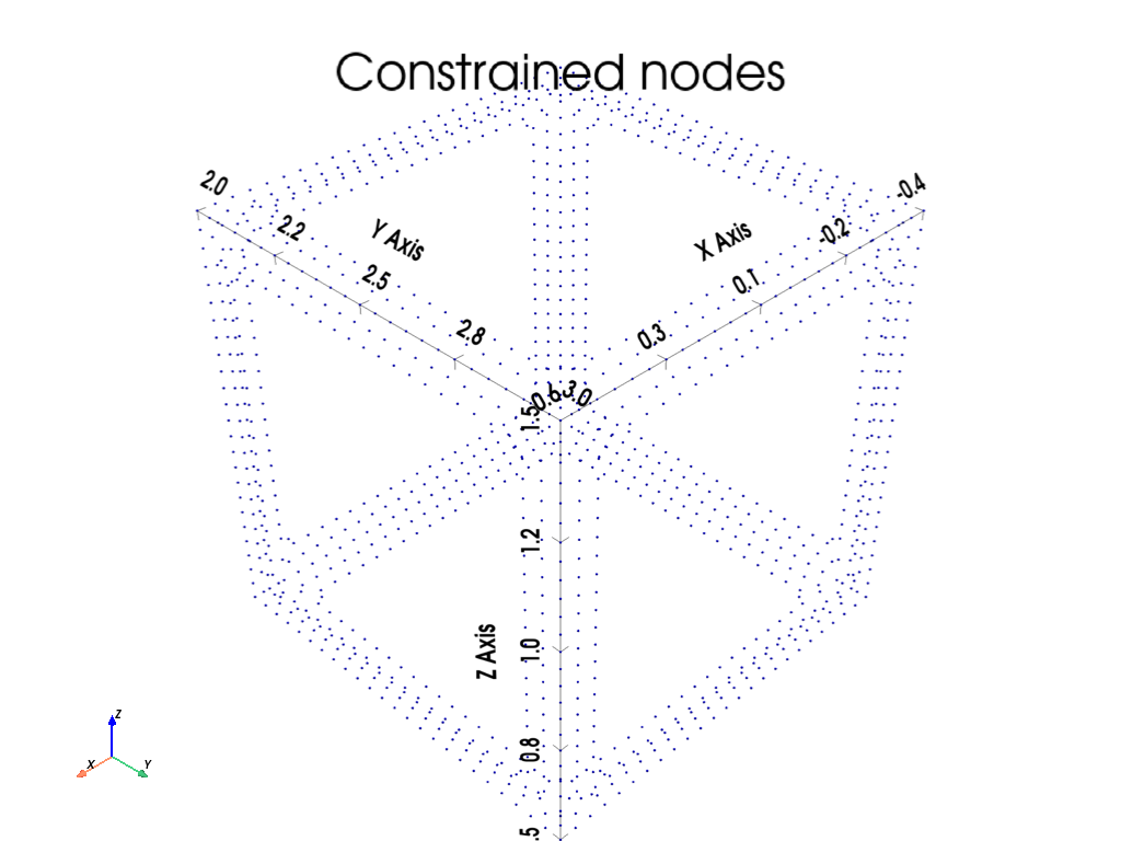
# Plot boundary nodes of the local model
mapdl.nplot(background="w", color="b", show_bounds=True, title="Constrained nodes")
# Exit PREP7
mapdl.finish()
return boundary_coordinates
# Define the boundary conditions and the loading for the global model
define_bcs(mapdl_global)
# Get the DPF field with the boundary nodes of the local model
boundary_coords = get_boundary(mapdl_local)
Set up DPF operators#
We define two DPF operators: the first reads the displacement results from the global model,
and the second interpolates those displacements onto the boundary coordinates of the local
model. The DataSources class to link results with the DPF operator inputs.
def define_dpf_operators(n_cores):
    """
    Define DPF operators for the global model.

    Parameters
    ----------
    n_cores : int
        Number of cores used in the global model.

    Returns
    -------
    dpf.Model
        DPF model for the global model.
    dpf.Operator
        DPF operator to read nodal displacements from the global model.
    dpf.Operator
        DPF operator to interpolate displacements onto local model boundary coordinates.
    """
    # Define the DataSources class and link it to the results of the global model
    data_sources = dpf.DataSources()
    for i in range(n_cores):
        data_sources.set_domain_result_file_path(
            path=Path(f"./outputs/mapdl-dpf/global/file{i}.rst"), key="rst", domain_id=i
        )

    global_model = dpf.Model(data_sources)
    # Define displacement result operator to read nodal displacements
    global_disp_op = dpf.operators.result.displacement()
    # Connect displacement result operator with the global model's results file
    global_disp_op.inputs.data_sources.connect(data_sources)
    # Define interpolator to interpolate the results inside the mesh elements
    # with shape functions
    disp_interpolator = dpf.operators.mapping.on_coordinates()
    return global_model, global_disp_op, disp_interpolator


def initialize_dpf_interpolator(
    global_model,
    local_bc_coords,
    disp_interpolator,
):
    """
    Initialize the DPF interpolator for the local model.

    Parameters
    ----------
    global_model : dpf.Model
        DPF model for the global model.
    local_bc_coords : dpf.Field
        DPF field containing the coordinates of the boundary nodes of the local model.
    disp_interpolator : dpf.Operator
        DPF operator to interpolate displacements onto local model boundary coordinates.
    """
    my_mesh = global_model.metadata.meshed_region  # Global model's mesh
    disp_interpolator.inputs.coordinates.connect(
        local_bc_coords
    )  # Link interpolator inputs with the local model's boundary coordinates
    disp_interpolator.inputs.mesh.connect(
        my_mesh
    )  # Link interpolator mesh with the global model's mesh


def interpolate_data(timestep):
    global_disp_op.inputs.time_scoping.connect(
        [timestep]
    )  # Specify timestep value to read results from
    global_disp = (
        global_disp_op.outputs.fields_container.get_data()
    )  # Read global nodal displacements

    disp_interpolator.inputs.fields_container.connect(
        global_disp
    )  # Link the interpolation data with the interpolator
    local_disp = disp_interpolator.outputs.fields_container.get_data()[
        0
    ]  # Get displacements of the boundary nodes of the local model
    return local_disp


# Define the two DPF operators
global_model, global_disp_op, disp_interpolator = define_dpf_operators(n_cores)
Set up simulation loop#
We solve the two models sequentially for each loading step. First the global model is run producing a .rst results file. Then we extract the global displacements and use them to define cut-boundary conditions for the local model (an input string command will be used for faster excecution time).
def define_cut_boundary_constraint_template(local_bc_coords):
    """
    Define template of input string command to apply the displacement constraints.

    Parameters
    ----------
    local_bc_coords : dpf.Field
        DPF field containing the coordinates of the boundary nodes of the local model.

    Returns
    -------
    str
        Template of input string command to apply the displacement constraints.
    """
    # Define template of input string command to apply the displacement constraints
    local_nids = local_bc_coords.scoping.ids
    # Get Node ID of boundary nodes of the local model
    template = ""
    for nid in local_nids:
        template += (
            "d,"
            + str(nid)
            + ",ux,{:1.6e}\nd,"
            + str(nid)
            + ",uy,{:1.6e}\nd,"
            + str(nid)
            + ",uz,{:1.6e}\n"
        )
    return template


def solve_global_local(mapdl_global, mapdl_local, timesteps, local_bc_coords):
    """
    Solve the global and local models sequentially for each timestep.

    Parameters
    ----------
    mapdl_global : Mapdl
        MAPDL instance for the global model.
    mapdl_local : Mapdl
        MAPDL instance for the local model.
    timesteps : int
        Number of timesteps to solve.
    local_bc_coords : dpf.Field
        DPF field containing the coordinates of the boundary nodes of the local model.
    """
    # Enter solution processor
    mapdl_global.solution()
    mapdl_local.solution()

    # Static analysis
    mapdl_global.antype("STATIC")
    mapdl_local.antype("STATIC")

    constraint_template = define_cut_boundary_constraint_template(local_bc_coords)

    for i in range(1, timesteps + 1):  # Iterate timesteps
        print(f"Timestep: {i}")
        st = tt.time()
        # Set loadstep time for the global model
        mapdl_global.time(i)
        # No extrapolation
        mapdl_global.eresx("NO")
        mapdl_global.allsel("ALL")
        # Write ALL results to database
        mapdl_global.outres("ALL", "ALL")
        # Solve global model
        mapdl_global.solve()
        print("Global solve took ", tt.time() - st)

        # Initialize interpolator
        if i == 1:
            initialize_dpf_interpolator(global_model, local_bc_coords, disp_interpolator)
        # Read  & Interpolate displacement data
        local_disp = interpolate_data(timestep=i)
        # Run MAPDL input string command to apply the displacement constraints
        data_array = np.array(local_disp.data).flatten()
        mapdl_local.input_strings(constraint_template.format(*data_array))

        st = tt.time()
        mapdl_local.allsel("ALL")
        # Set loadstep time for the local model
        mapdl_local.time(i)
        # No extrapolation
        mapdl_local.eresx("NO")
        # Write ALL results to database
        mapdl_local.outres("ALL", "ALL")
        # Solve local model
        mapdl_local.solve()
        print("Local solve took ", tt.time() - st)

    # Exit solution processor
    mapdl_global.finish()
    mapdl_local.finish()
Solve system#
Timestep: 1
Global solve took  0.29200077056884766
Local solve took  0.5194289684295654
Timestep: 2
Global solve took  0.29796671867370605
Local solve took  0.47373461723327637
Timestep: 3
Global solve took  0.24790430068969727
Local solve took  0.430649995803833
Timestep: 4
Global solve took  0.26927852630615234
Local solve took  0.47283005714416504
Timestep: 5
Global solve took  0.24740147590637207
Local solve took  0.478381872177124
Timestep: 6
Global solve took  0.2483806610107422
Local solve took  0.4309530258178711
Timestep: 7
Global solve took  0.26798391342163086
Local solve took  0.43282318115234375
Timestep: 8
Global solve took  0.2546544075012207
Local solve took  0.43082666397094727
Timestep: 9
Global solve took  0.26779699325561523
Local solve took  0.432755708694458
Timestep: 10
Global solve took  0.2811872959136963
Local solve took  0.4760899543762207
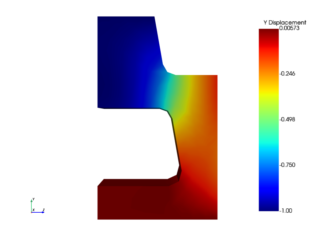
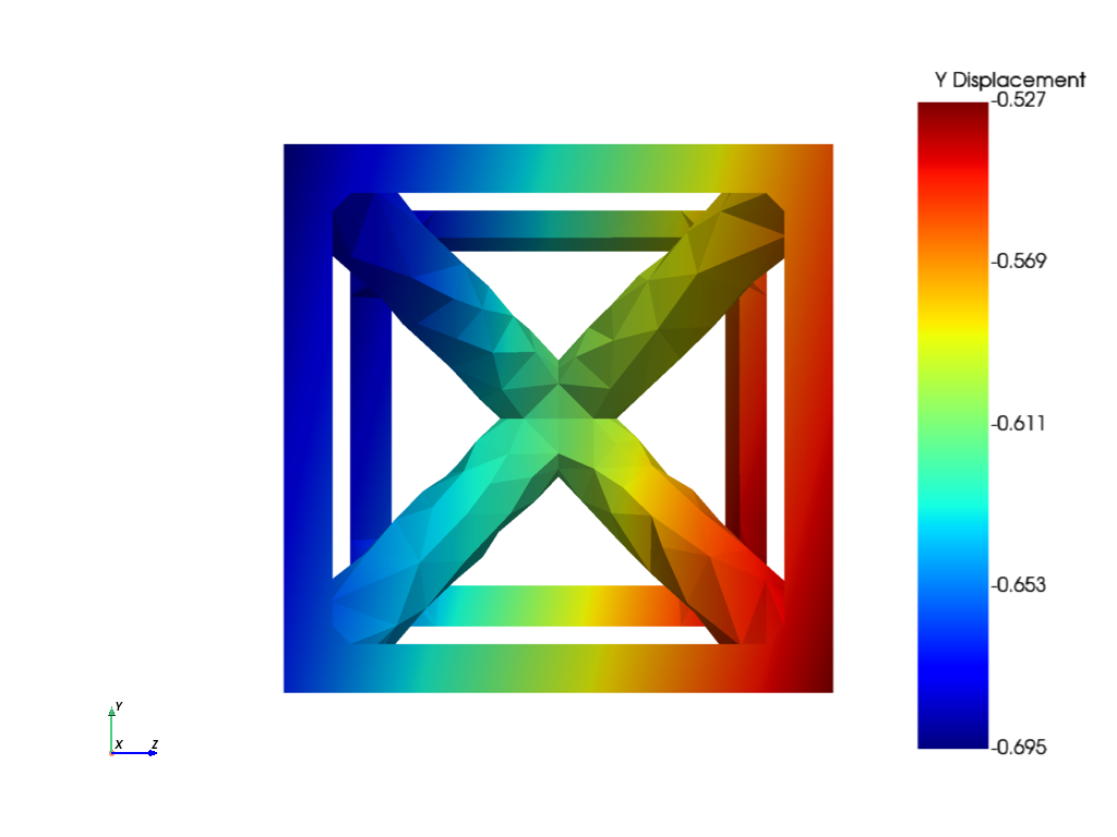
Visualize results#
def visualize(mapdl):
    # Enter post-processing
    mapdl.post1()
    # Set the current results set to the last set to be read from result file
    mapdl.set("LAST")
    # Plot nodal displacement of the loading direction
    mapdl.post_processing.plot_nodal_displacement("Y", cmap="jet", background="w", cpos="zy")
    # Exit post-processing
    mapdl.finish()


# Plot Y displacement of global model
visualize(mapdl_global)

# Plot Y displacement of local model
visualize(mapdl_local)
Exit MAPDL instances#
mapdl_pool.exit()
Total running time of the script: (0 minutes 18.785 seconds)